I also had a close encounter with this body of work. It is nice to know that i am not the only mathematician so intrigued.
Far too often mathematics or at least some particular problem really fires up the juices of obscession. This does not mean that the problem is solvable. Often it just looks like it. Fermats last Theorem is one such.
I discovered there that the far more interesting question was to understand why Fermat got excited at all
The Riemann Hypothesis, explained
Nov 12
Eight years ago, in 2013, I wrote an undergraduate thesis entitled ‘Prime Numbers and the Riemann Zeta Function’. About three years later, I published a condensed version as an article on Medium, entitled ‘The Riemann Hypothesis, explained’. That article was later picked up on Hacker News, where it ended up on the front page. Because of that exposure, the article eventually became one of the top Google results for the search term ‘The Riemann Hypothesis’. When Michael Atiyah (1929-2019) later claimed to have solved the RH, the magazine Science contacted me to comment on this claim (probably because the journalist searched ‘The Riemann Hypothesis’ and found my article). My statements from the article that journalist wrote eventually ended up in news outlets around the world (including The Times, USA Today, the New York Post and many others). From that exposure and the traffic it generated, I was later contacted by Medium about launching a digital magazine focused on mathematics and physics. Founding that magazine, called Cantor’s Paradise, is how I eventually came to start writing Privatdozent.
So, I figure this is where I come full circle. My writing has hopefully improved in the last eight years, but most of the analysis is still up to date. The article assumes an undergraduate-level understanding of mathematics.
This week I present to you, the Riemann hypothesis, explained.
Introduction
The properties of the prime numbers have been studied by many of history’s mathematical giants. From the first proof of the infinity of the primes by Euclid, to Euler’s product formula which connected the prime numbers to the zeta function. From Gauss and Legendre’s formulation of the prime number theorem to its proof by Hadamard and de la Vallée Poussin. Bernhard Riemann still reigns as the mathematician who made the single biggest breakthrough in prime number theory. His work, all contained in an eight page paper published in 1859 made new and previously unknown discoveries about the distribution of the primes and is to this day considered to be one of the most important papers in number theory.
Since its publication, Riemann’s paper has been the main focus of prime number theory and was indeed the main reason for the proof of something called the prime number theorem in 1896. Since then several new proofs have been found, including elementary proofs by Selberg and Erdós. Riemann’s hypothesis about the roots of the zeta function however, remains a mystery.
How many Primes there?
Let’s start off easy. We all know that a number is either prime or composite. All composite numbers are made up of, and can be broken down (factorized) into a product (a x b) of prime numbers. Prime numbers are in this way the “building blocks” or “fundamental elements” of numbers. They were proven to be infinite in number by Euclid, 300 years BCE. His elegant proof goes as follows:
Euclid’s Theorem. Assume that the set of prime numbers is not infinite. Make a list of all the primes. Next, let P be the product of all the primes in the list (multiply all the primes in the list). Add 1 to the resulting number, Q = P +1. As with all numbers, this number Q has to be either prime or composite:
- If Q is prime, you’ve found a prime that was not in your “list of all the primes”.
- If Q is not prime, it is composite, i.e made up of prime numbers, one of which, p, would divide Q (since all composite numbers are products of prime numbers). Every prime p that makes up P obviously divides P. If p divides both P and Q, then it would have to also divide the difference between the two, which is 1. No prime number divides 1, and so the number p cannot be on your list, another contradiction that your list contains all prime numbers.
There will always be another prime p not on the list which divides Q. Therefore there must be infinitely many primes numbers.
Why are Primes so Hard to Understand?
The mere fact that any novice understands the problem I laid out above, speaks volumes about how difficult it is. Even the arithmetic properties of primes, while heavily studied, are still poorly understood. The scientific community is so confident in our lacking ability to understand how prime numbers behave that the factorization of large numbers (figuring out which two primes multiply together to make a number) is one of the the very foundations of encryption theory. Here’s one way of looking at it:
We understand composite numbers well. Those are all the non-primes. They are made up of primes, but you can easily write a formula that predicts and/or generates composites. Such a “composite filter” is called a sieve. The most famous example is named the “Sieve of Eratosthenes” from c. 200 BCE. What it does, is simply mark the multiples of each prime up to a set limit. So, take the prime 2, and mark 4,6,8,10 and so on. Next, take 3, and mark 6,9,12,15 and so on. What you’ll be left with is only primes. Although very simple to understand, the sieve of Erathosthenes is as you can imagine, not very efficient.
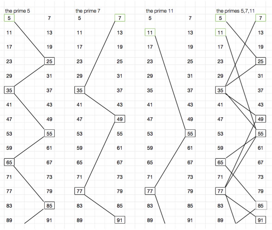
One function simplifying your work significantly is 6n +/- 1. This simple function spits out all primes except 2 and 3, and removes all multiples of 3 and all even numbers. Put in for n = 1, 2, 3, 4, 5, 6, 7 and behold the result: 5, 7, 11, 13, 17, 19, 23, 25, 29, 31, 35, 37, 41, 43. The only non-prime numbers generated by the function are 25 and 35, which can be factorized into 5 x 5 and 5 x 7, respectively. The next non-primes are, as you can imagine, 49 = 7 x 7, 55 = 5 x 11 and so on. Simple right?
Illustrating this visually, I’ve used something that I’m calling “composite ladders”, a simple way to see how the composite numbers generated by the function are laid out for each prime, and combined. In the first three columns of the image below, you neatly see the prime numbers 5, 7 and 11 with each respective composite ladder up to and including 91. The chaos of the fourth column, showing how the sieve has removed all but the prime numbers, is a fair illustration of why prime numbers are so hard to understand.
Fundamental Resources
So what does this all have to do with this thing you may have heard of called the “Riemann hypothesis”? Well, said simply, in order to understand more about primes, mathematicians in the 1800s stopped trying to predict with absolute certainty where a prime number was, and instead started looking at the phenomenon of prime numbers as a whole. This analytic approach is what Riemann was a master of, and where his famous hypothesis was made. Before I can explain it however, it is necessary to get familiar with some fundamental resources.
The Harmonic Series
The harmonic series is an infinite series of numbers first studied by Nicholas Oresme in the 14th century. Its name relates to the concept of harmonics in music, overtones higher than the fundamental frequency of a tone. The series is as follows:

The first terms of the infinite harmonic series
This sum was proven to be divergent by Oresme (not having a finite limit, not approaching/tending towards any particular number, but running off into infinity).
Zeta Functions
The harmonic series is a special case of a more general type of function called a zeta function ζ(s). The real valued zeta function is given for r and n, two real numbers:

The Zeta Function
If you put in for n = 1, you get the harmonic series, which diverges. For all values of n > 1 however, the series converges, meaning the sum tends towards some number as the value of r increases, i.e it does not run off into infinity.
The Euler Product Formula
The first connection between zeta functions and prime numbers was made by Euler when he showed that for n and p, two natural numbers (integers larger than zero) where p is prime:

The Euler Product Formula for two numbers n, p where both are larger than zero and p is a prime number
This expression first appeared in a paper in 1737 entitled Variae observationes circa series infinitas. The expression states that the sum of the zeta function is equal to the product of the reciprocal of one minus the reciprocal of primes to the power s. This astonishing connection laid the foundation for modern prime number theory, which from this point on used the zeta function ζ(s) as a way of studying primes.
The proof of the formula is one of my favorites, and so I will include iteven though it is not strictly necessary for our purposes (it’s just so lovely!):
Proof of Euler’s Product Formula
Euler begins with the general zeta function
First, he multiplies both sides by the second term:
He then subtracts the resulting expression from the zeta function:
The zeta function minus 1/2^s times the zeta function
He repeats this process, next multiplying both sides by the third term
The zeta function minus 1/2^s times the zeta function, multiplied by 1/3^s
And then subtracting the resulting expression from the zeta function
The zeta function minus 1/2^s times the zeta function minus 1/3^s times the zeta function
Repeating this process to infinity, one would in the end be left with the expression:

1 minus all the prime reciprocals, multiplied by the zeta function
If this process is familiar to you, it is because what Euler constructed was in fact, a sieve, much like the Sieve of Eratosthenes. He is filtering out non-prime numbers from the zeta function.
Next, divide the expression by all of the prime reciprocal terms, and obtain:

Shortened, we have shown that:

The Euler product formula, the identity which shows the connection between prime numbers and the zeta function
Wasn’t that beautifully done? Put in for s = 1, and find the infinite harmonic series, re-proving the infinity of the primes.
The Möbius Function
August Ferdinand Möbius later rewrote the Euler product formula to create a new sum. In addition to containing reciprocals of primes, Möbius’ function also contains every natural number that is the product of odd and even numbers of prime factors. The numbers left out of his series are those that divide by some prime squared. His sum, denoted by μ(n) is as follows:

The Möbius function, an altered version of Euler’s Product Formula, defined for all natural numbers
The sum contains reciprocals of:
Every prime;
Every natural number which is a product of an odd number of different primes, prefixed by a minus sign; and
Every natural number that is the product of an even number of different primes, prefixed by a plus sign;
Below are the first terms:

The series/sum of 1 divided by the zeta function ζ(s)
The sum does not contain reciprocals of numbers which divide by some prime squared, e.g 4,8,9 and so on.
The Möbius function μ(n) only takes on three possible values which either prefix (1 or -1) or remove (0) terms from the sum:

The three possible values of the Möbius function μ(n)
Although first formally defined by Möbius, this quirky sum was remarkably considered by Gauss in a sidenote more than 30 years earlier, when he wrote:
“The sum of all primitive roots (of a prime number p) is either ≡ 0 (when p-1 is divisible by a square), or ≡ ±1 (mod p) (when p-1 is the product of unequal prime numbers); if the number of these is even the sign is positive, but if the number is odd, the sign is negative.”
The Prime Counting Function
Back to primes. To understand how primes are distributed as you go higher up the number line, without knowing where they are, it is useful to instead count how many there are up to a certain number.
The prime counting function π(x), introduced by Gauss, does just that, gives the number of primes less than or equal to a given real number. Given that there is no known formula for finding primes, the prime counting formula is known to us only as a plot, or step function increasing by 1 whenever x is prime. The plot below shows the function up to x = 200.
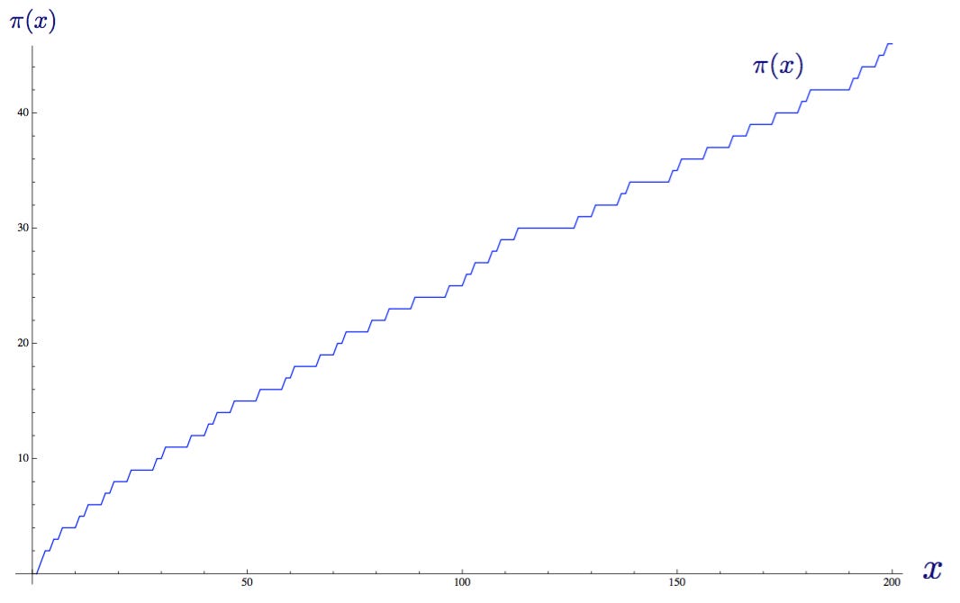
The prime counting function π(x) up to x = 200.
The Prime Number Theorem
The prime number theorem, also formulated by Gauss (and Legendre, independently) states:

The Prime Number Theorem
In English, it states: “As x goes to infinity, the prime counting function π(x) will approximate the function x/ln(x)”. In other words, if you count high enough, and plot the number of primes up to a very large number x, then plot x divided by the natural logarithm of x, the ratio between the two will approach 1. The two functions are plotted below for x = 1000:
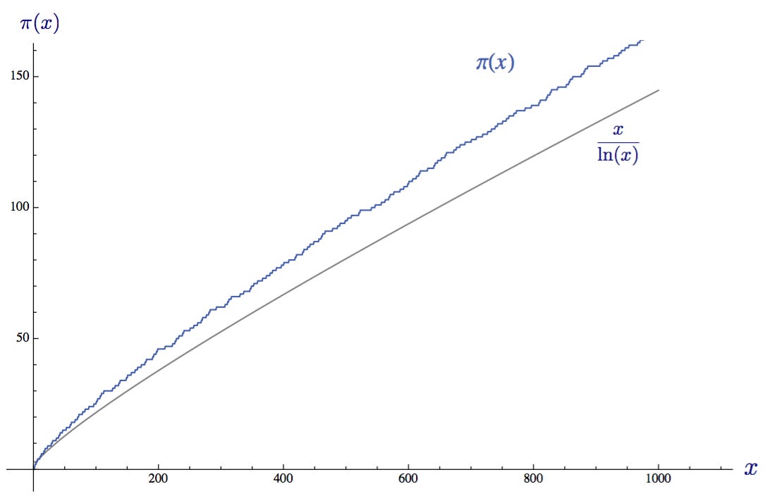
The prime counting function π(x) and the estimate from the prime number theorem plotted up to x = 1000
In terms of probability, the prime number theorem states that if you pick a natural number x at random, the probability P(x) that that number will be a prime number is about 1 / ln(x). This means that the average gap between consecutive prime numbers among the first x integers is approximately ln(x).
The Logarithmic Integral Function
The function Li(x) is defined for all positive real numbers exceptx = 1. It is defined by an integral from 2 to x:

The integral representation of the logarithmic integral function
Plotting this function alongside the prime counting function and the formula from the prime number theorem, we see that Li(x) is actually a better approximation than x/ln(x):
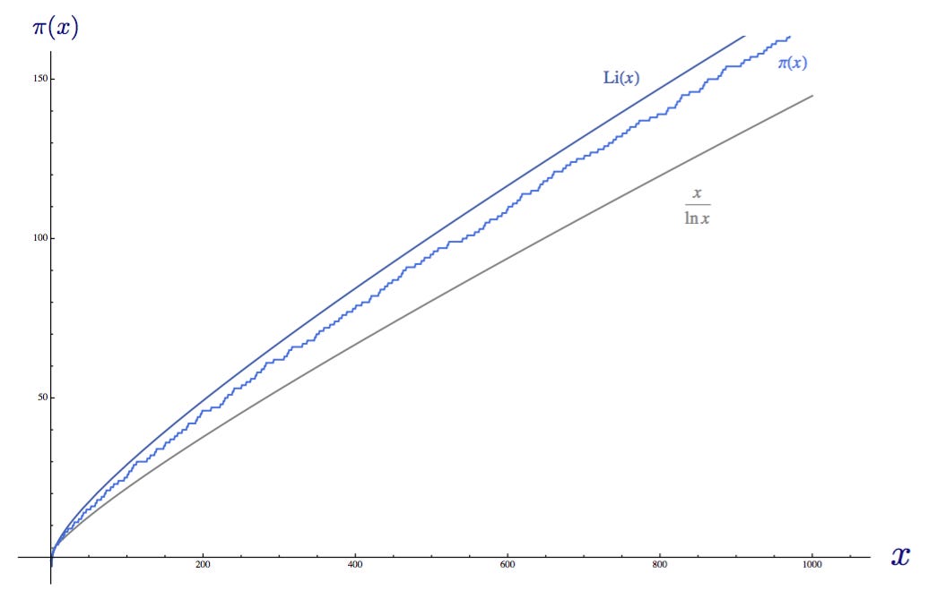
The logarithmic integral function Li(x), the prime counting function π(x) and x/ln(x) plotted together
How much better of an approximation it is, can be seen if we make a table with large values of x, the number of primes up to x and the error of the old (prime number theorem) and new (logarithmic integral) functions:
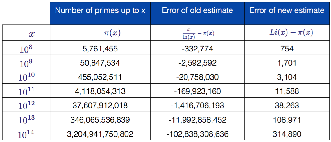
The number of primes up to a given power of ten and corresponding error terms for the two estimates
As can be easily seen here, the logarithmic integral function is far better of an approximation than the function from the prime number theorem, only “overshooting” by 314,890 primes for x = 10 to the power of 14. However, both functions do converge towards the prime counting function π(x). Li(x)does so much faster, but as x goes to infinity, the ratio between the prime counting function and both functions Li(x) and x/ln(x) goes towards 1. Visualized:
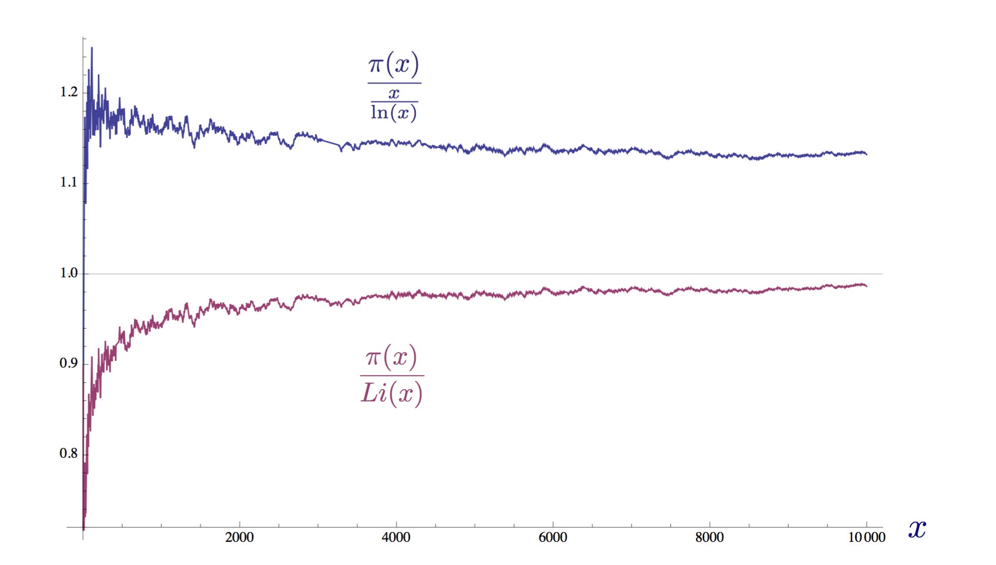
Convergence of the ratios of the two estimates and the prime counting function towards 1 with x = 10,000
The Gamma Function
The gamma function Γ(z) has been an important object of study since the problem of extending the factorial function to non-integer arguments was studied by Daniel Bernoulli and Christian Goldbach in the 1720s. It is an extension of the factorial function n! (1 x 2 x 3 x 4 x 5 x …. n), shifted down by 1:

The gamma function, defined for z
Its plot is very curious:
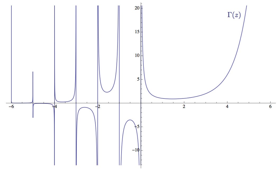
The Gamma Function Γ(z) plotted in the range -6 ≤ z ≤ 6
The gamma function Γ(z)is defined for all complex values of z larger than zero. Complex numbers, as you probably know, are a class of numbers with an imaginary part, written as Re(z) + Im(z), where Re(z) is the real part (ordinary real number) and Im(z) is the imaginary part, denoted by the letter i. A complex number is typically written in the form z = σ + it where sigma σ is the real part and it is the imaginary part. Complex numbers are useful because they allow mathematicians and engineers to evaluate and work on problems where ordinary real numbers will not allow it. Visualized, complex numbers extend the traditional one-dimensional “number line” into a two-dimensional “number plane”, called the complex plane, in which the real part of a complex number is plotted on the x-axis and the imaginary part is plotted on the y-axis.
In order to be able to use the gamma function Γ(z), it is typically rewritten to the form

The functional relationship of the gamma function Γ(z)
Using this identity, one can obtain values for z below zero. It does not however give values for negative integers, as they are not defined (technically they are singularities, or simple poles).
Zeta and Gamma
The link between the zeta function and the gamma function is given by the following integral:

Bernhard Riemann
Now that we’ve covered the necessary fundamental resources, we can finally begin making the connection between prime numbers and the Riemann Hypothesis.
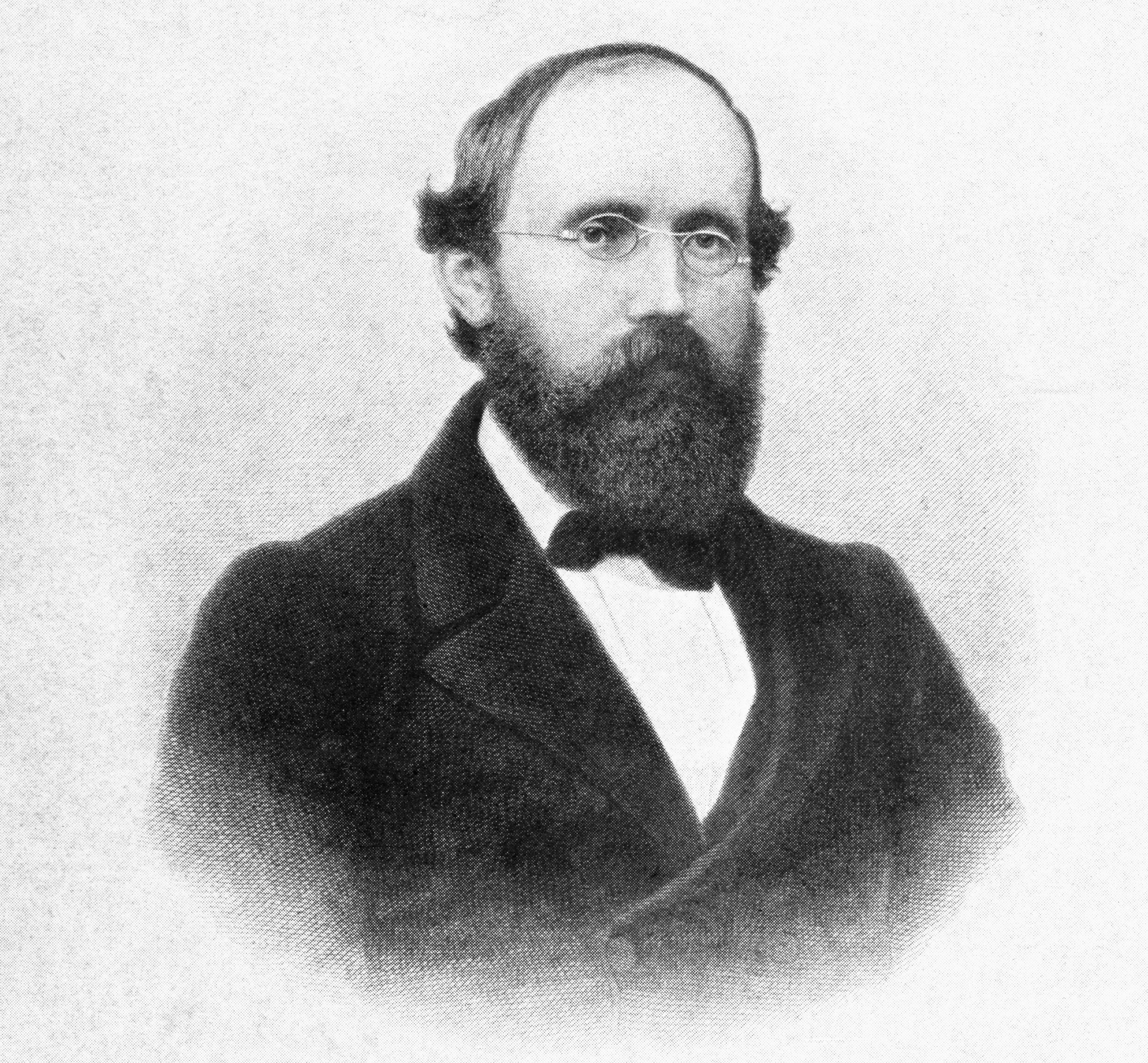
German mathematician Bernhard Riemann was born in Breselenz in 1826. Student of Gauss, Riemann published work in the fields of analysis and geometry. His biggest contribution was likely in the field of differential geometry, where he laid the groundwork for the geometric language later used in Einstein’s General Theory of Relativity.
His sole effort in number theory, the 1859 paper Ueber die Anzahl der Primzahlen unter einer gegebenen Grösse, “On prime numbers less than a given magnitude” is considered the most important paper in the field. In four short pages he outlined:
A definition of the Riemann zeta function ζ(s), a complex-valued zeta function;
The analytic continuation of the zeta function to all complex numbers s≠1;
A definition for the Riemann xi function ξ(s), an entire function related to the Riemann zeta function through the gamma function;
Two proofs of the functional equation of the Riemann zeta function;
A definition of the Riemann prime counting function J(x) by using the prime counting function and the Möbius function;
An explicit formula for the number of primes less than a given number by using the Riemann prime counting function, defined using the non-trivial zeros of the Riemann zeta function.
An incredible feat of engineering and creativity, the likes of which probably hasn’t been seen since. Absolutely astounding.
The Riemann Zeta Function
We’ve seen the intimate relationship between prime numbers and the zeta function shown by Euler in his product formula. Beyond this connection however, not much was known about the relationship and it would take the invention of complex numbers to show explicitly just how interconnected the two are.
Riemann was the first to consider the zeta function ζ(s) for a complex variable s, where s = σ + it.

The Riemann Zeta Function for nwhere s = σ + it is a complex number where both σ and t are real numbers.
Dubbed the Riemann zeta function ζ(s), it is an infinite series which is analytic (has definable values) for all complex numbers with real part larger than 1 (Re(s) > 1). In this area, it converges absolutely.
In order to analyze the function in areas beyond the regular area of convergence (when the real part of the complex variable s is larger than 1), the function needs to be redefined. Riemann successfully does this by analytic continuation to an absolutely convergent function in the half plane Re(s) > 0.

The rewritten form of the Riemann zeta function, where {x} = x — |x|
This new definition for the zeta function is analytic everywhere in the half plane Re(s) > 0, except at s = 1 where there is a singularity/simple pole. This is called a meromorphic function in this domain, because it is holomorphic (complex differentiable in a neighborhood of every point in its domain) except for at the simple pole s = 1. It is also a great example of something called a Dirichlet L-function.
In his paper, Riemann does not stop there. He goes on to analytically continue his zeta function ζ(s) to the entire complex plane, using the gamma function Γ(z). In the interest of keeping this article simple, I will not show this calculation here, but I strongly urge you to read it for yourself as it demonstrates Riemann’s remarkable intuition and technique supremely well (edit 03.13.20: the calculation is available in Veisdal (2013) pp. 28).
His method makes use of the integral representation of gamma Γ(z) for complex variables and something called the Jacobi theta function ϑ(x), which together can be rewritten so that the zeta function appears. Solving for zeta,

A functional zeta equation for the entire complex plane except two singularities at s = 0 and s = 1
In this form, one can see that the term ψ(s) decreases more rapidly than any power of x, and so the integral converges for all values of s.
Going even further, Riemann notices that the first term in the braces (-1 / s(1 - s) ) is invariant (does not change) if one substitutes s by 1 - s. Doing so, Riemann further extends the usefulness of the equation byremoving the two poles at s=0 and s=1, and defining the Riemann xi function ξ(s) with no singularities:

The Riemann xi function ξ(s)
Zeros of the Riemann Zeta Function
The roots/zeros of the zeta function, when ζ(s)=0, can be divided into two types which have been dubbed the “trivial” and the “non-trivial” zeros of the Riemann zeta function.
Existence of zeros with real part Re(s) < 0
The trivial zeros are the zeros which are easy to find and explain. They are most easily noticable in the following functional form of the zeta function:

A variation of Riemann’s functional zeta equation
This product becomes zero when the sine term becomes zero. It does so at kπ. So, e.g for a negative even integer s = -2n, the zeta function becomes zero. For positive even integers s = 2n however, the zeros are cancelled out by the poles of the gamma function Γ(z). This is easier to see in the original functional form, where if you put in for s = 2n, the first part of the term becomes undefined.

So, the Riemann zeta function has zeros at every negative even integer s = -2n. These are the trivial zeros, and they can be seen in the plot of the function below:
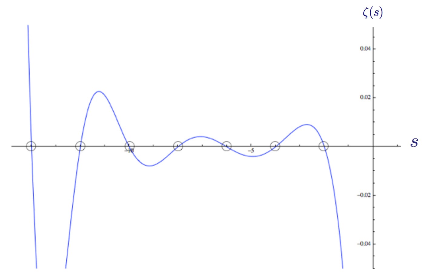
The Riemann zeta function ζ(s) plotted with the trivial zeros highlighted at s= -2, -4, -6 and so on
Existence of zeros with real part Re(s) > 1
From Euler’s product formulation of zeta, we can immediately see that zeta ζ(s) cannot be zero in the area with real part of s larger than 1 because a convergent infinite product can only be zero if one of its factors is zero. The proof of the infinity of the primes denies this.

The Euler Product Formula
Existence of zeros with real part 0 ≤ Re(s) ≤ 1
We’ve now found the trivial zeros of zeta in the negative half plane when Re(s) < 0 and shown that there cannot be any zeros in the area Re(s) > 1.
The area between these two areas however, called the critical strip, is where much of the focus of analytic number theory has taken place for the last few hundred years.
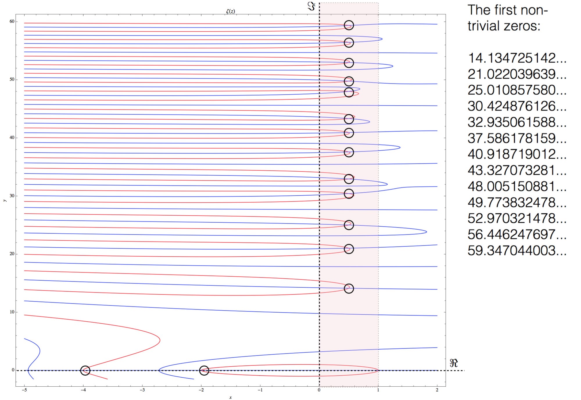
Plot of the real and imaginary part of the Riemann zeta function ζ(s) in the interval -5 < Re < 2, 0 < Im < 60
In the plot above I have graphed the real parts of zeta ζ(s) in red and the imaginary parts in blue. We see the first two trivial zeros in the lower left when the real part of s is -2 and -4. In between 0 and 1, I have highlighted the critical strip and marked off where the real and imaginary parts of zeta ζ(s) intersect. These are the non-trivial zeros of the Riemann zeta function. Going to higher values we see more zeros, and two seemingly random functions which appear to be getting denser as the imaginary part of s gets larger.
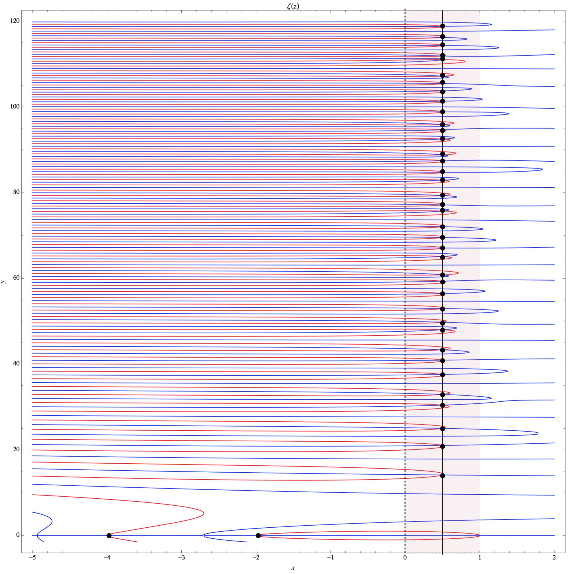
Plot of the real and imaginary parts of the Riemann zeta function ζ(s) in the interval -5 < Re < 2, 0 < Im < 120
The Riemann Xi Function
We’ve defined the Riemann Xi function ξ(s) (the version of the functional equation which has removed the singularities, and so is defined for all values of s) as:

The Riemann Xi function (no singularities)
This function satisfies the relationship

Symmetric relationship between the positive and negative values of the Riemann Xi function
Which means that the function is symmetric about the vertical line Re(s) = 1/2 so that ξ(1) = ξ(0), ξ(2) = ξ(-1) and so on. This functional relationship (the symmetry of s and 1-s) combined with the Euler product formula shows that the Riemann xi function ξ(s) can only have zeros in the range 0 ≤ Re(s) ≤ 1. The zeros of the Riemann xi function in other words correspond to the non-trivial zeros of the Riemann Zeta function. In a sense, the critical line R(s) = 1/2 for the Riemann Zeta function ζ(s) corresponds to the real line (Im(s) = 0) for the Riemann xi function ξ(s).
Looking at the two charts above, one should immediately take note of the fact that all the non-trivial zeros of the Riemann Zeta function ζ(s) (the zeros of the Riemann xi function) have real part Re(s) equal to 1/2. Riemann briefly remarked on this phenomenon in his paper, a fleeting comment which would end up as one of his greatest legacies.
The Riemann Hypothesis
The non-trivial zeros of the Riemann zeta function ζ(s) have real part Re(s) = 1/2.
This is the modern formulation of the unproven conjecture made by Riemann in his famous paper. In words, it states that the points at which zeta is zero, ζ(s) = 0, in the critical strip 0 ≤ Re(s) ≤ 1, all have real part Re(s) = 1/2. If true, all non-trivial zeros of Zeta will be of the form ζ(1/2 + it).
An equivalent statement (Riemann’s actual statement) is that all the roots of the Riemann xi function ξ(s) are real.
In the plot below, the line Re(s) = 1/2 is the horizontal axis. The real part Re(s) of zeta ζ(s) is the red graph and the imaginary part Im(s) is the blue graph. The non-trivial zeros are the intersections between the red and blue graph on the horizontal line.
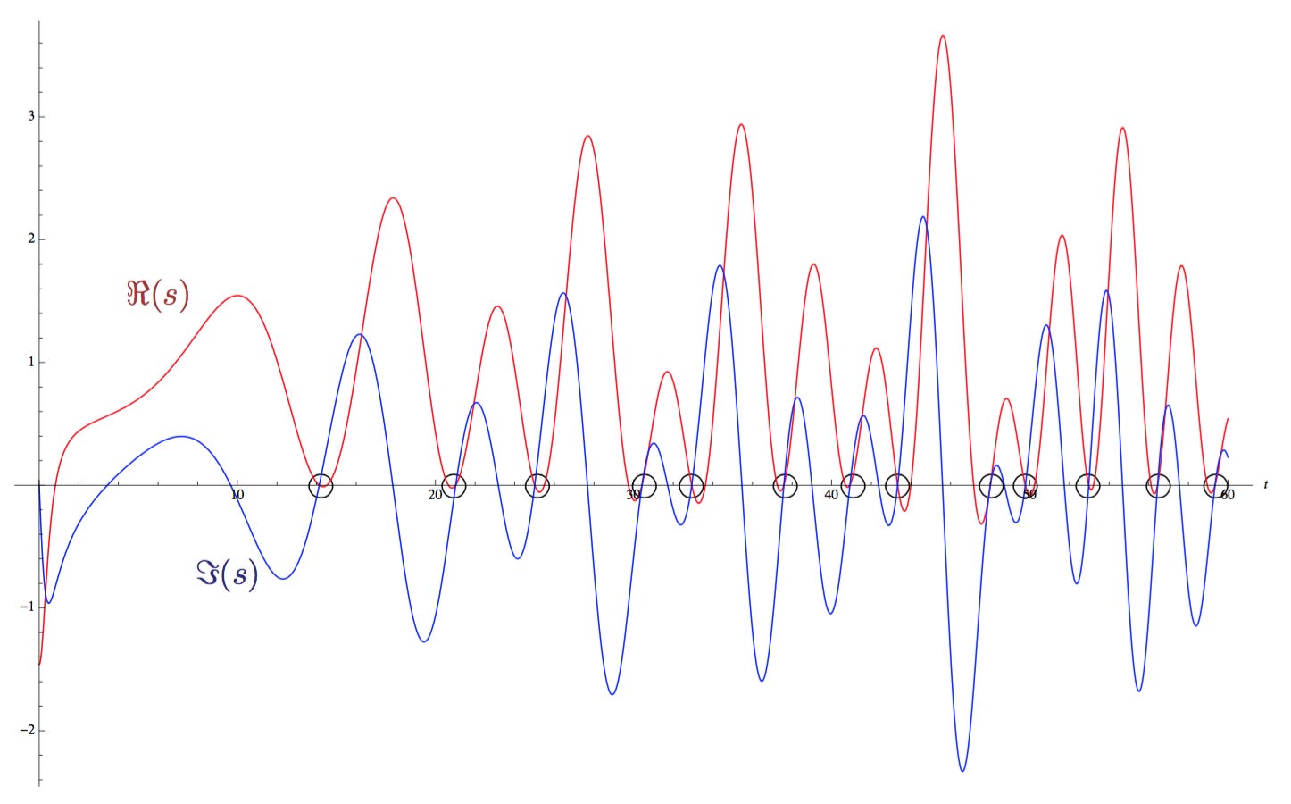
The first non-trivial zeros of the Riemann zeta function on the line Re(s) = 1/2.
If the Riemann hypothesis turns out to be true, all the non-trivial zeros of the function will appear on this line as intersections between the two graphs.
Reasons to Believe the Hypothesis
There are many reasons to believe the truth of Riemann’s hypothesis about the zeros of the zeta function. Perhaps the most compelling reason for mathematicians is the consequences it would have for the distribution of prime numbers. The numerical verification of the hypothesis to very high values suggests its truth. In fact, the numerical evidence for the hypothesis is far strong enough to be regarded as experimentally verified in other fields such as physics and chemistry. However, the history of mathematics contains several conjectures that had been shown numerically to very high values and still were proven false. Derbyshire (2004) tells the story of the Skewes number, a very very large number that gave an upper bound, proving the falsity of one of Gauss’ conjectures that the logarithmic integral Li(x) is always greater than the prime counting function. It was disproven by Littlewood without an example, and then shown to must fail above Skewes’ very, very large number ten to the power of ten, to the power of ten, to the power of 34, showing that even though Gauss’ idea had been proven to be wrong, an example of exactly where is far beyond the reach of numerical calculation even today. This could also be the case for Riemann’s hypothesis, which has “only” been verified up to ten to the power of twelve non-trivial zeros.
The Riemann Zeta Function and Prime Numbers
Using the truth of the Riemann hypothesis as a starting point, Riemann began studying its consequences. In his paper he writes; “…it is very probable that all roots are real. Of course one would wish for a rigorous proof here; I have for the time being, after some fleeting vain attempts, provisionally put aside the search for this, as it appears dispensable for the next objective of my investigation.” His next objective was relating the zeros of the zeta function to the prime numbers.
Recall the prime counting function π(x)which denotes the number of primes up to and including a real number x. Riemann used π(x) to define his own prime counting function, the Riemann prime counting function J(x). It is defined as:

The Riemann Prime Counting Function
The first thing to notice about this function is that it is not infinite. At some term, the counting function will be zero because there are no primes for x < 2. So, taking J(100) as an example, the function will be made up of seven terms because the eight term will include an eight root of 100, which is approximately equal to 1.778279.., so this prime counting term becomes zero and the sum becomes J(100) = 28.5333….
Like the prime counting function, the Riemann prime counting function J(x) is a step function which increases in value when:

The possible values of the Riemann prime counting function J(x)
To relate the value of J(x) to how many primes there are up to and including x, we recover the prime counting function π(x)by a process called Möbius inversion (which I will not show here). The resulting expression is

The Prime Counting function π(x) and its relationship with the Riemann Prime Counting funtion and the Möbius function μ(n)
Remembering that the possible values of the Möbius function are

The three possible values of the Möbius function μ(n)
This means that we can now write the prime counting function as a function of the Riemann prime counting function, giving us
The Prime Counting Function written as a function of the Riemann prime counting function for the first seven values of n
This new expression is still a finite sum because J(x) is zero when x < 2 because there are no primes less than 2.
If we now look at our example of J(100), we get the sum

The Prime Counting function for x = 100
Which we know to be the number of primes below 100.
Translating the Euler Product Formula
Riemann next uses the Euler product formula as a starting point and derives a method for analytically evaluating the prime numbers in the infinitesimal language of calculus. Starting with Euler:
The Euler product formula for the first five primes
By first taking the logarithm of both sides, then rewriting the denominators in the parenthesis, he derives the relationship
The logarithm of the Euler product formula, rewritten
Next, using the well known Maclaurin Taylor series, he expands each log term on the right hand side, creating an infinite sum of infinite sums, one for each term in the prime number series.

The Taylor expansion of the first four terms of the logarithm of the Euler product formula
Looking at one such term, e.g:

The second term in the Maclaurin expansion of 1/3^s
This term, and every other term in the calculation, represents part of the area under the J(x) function. Written as an integral:

Integral form of the second term in the Maclaurin expansion of 1/3^s
In other words, using the Euler product formula, Riemann showed that it is possible to represent the discrete prime counting step function as a continuous sum of integrals. Below our example term is shown as part of the area under the Riemann prime counting function graph.
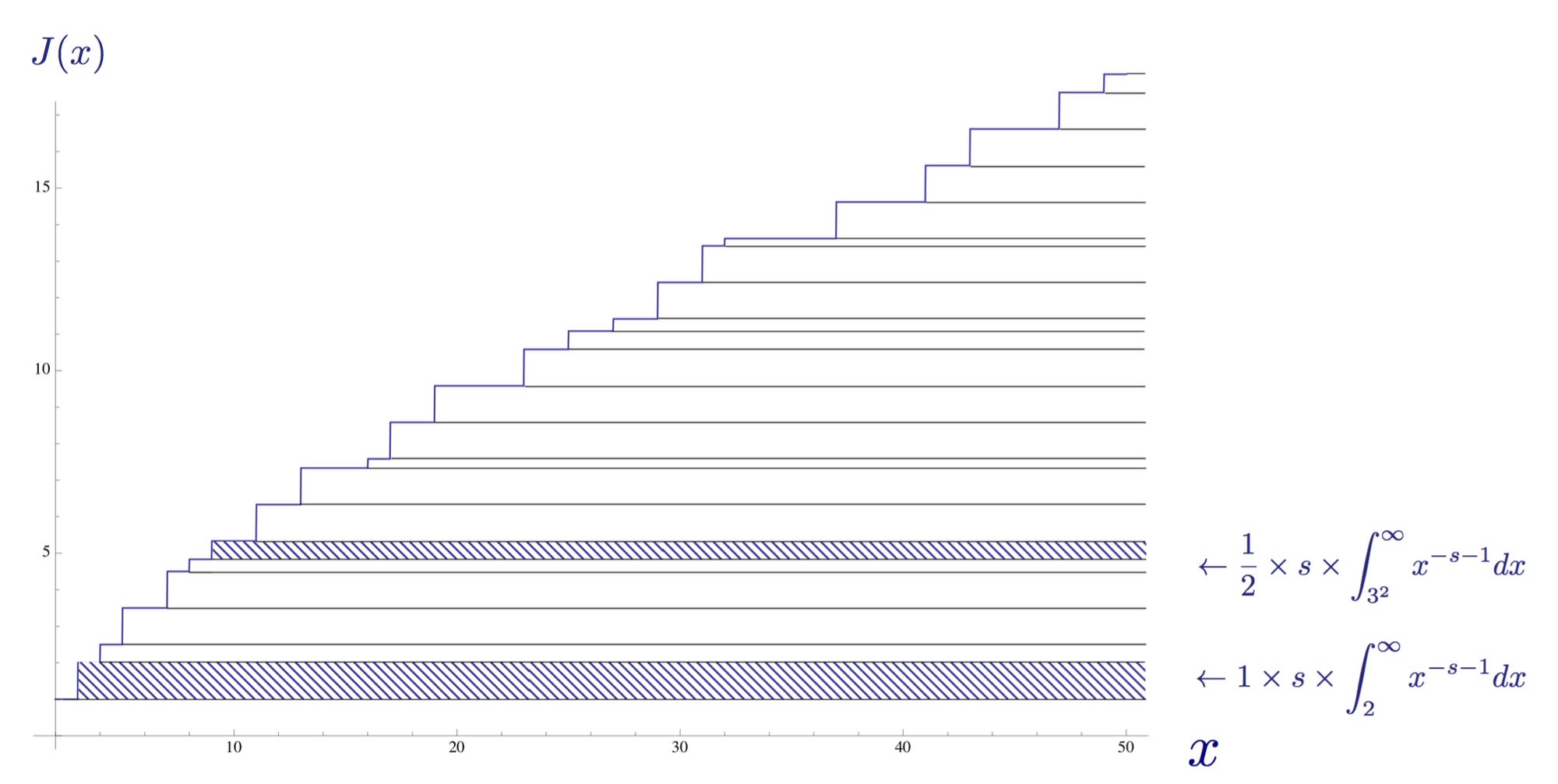
The Riemann Prime Counting function J(x) up to x = 50, with two integrals highlighted
So, each expression in the finite sum that makes up the prime reciprocal series of Euler product formula can be expressed as integrals, making an infinite sum of integrals that correspond to the area under the Riemann prime counting function. For the prime number 3, this infinite product of integrals is:
The infinite product of integrals making up the area under the prime counting function represented by the integer 3
Collecting all of these infinite sums together into one integral, the integral under the Riemann prime counting function J(x) can be written as simply:

The logarithm of zeta, expressed as an infinite series of integrals
Or, the more popular form

The modern equivalent of the Euler product formula, connecting the zeta function to the Riemann prime counting function
Riemann had with this connected his zeta function ζ(s) with his Riemann prime counting function J(x) in an identity statement equivalent to the Euler product formula, in the language of calculus.
The Error Term
Having obtained his analytic version of the Euler product formula, Riemann next went on to formulate his own prime number theorem. The explicit form he gave was:

“Riemann’s prime number theorem” guessing the number of primes under a given magnitude x
This is Riemann’s explicit formula. It is an improvement on the prime number theorem, a more accurate estimate of how many primes exist up to and including a number x. The formula has four terms:
The first term, or “principle term” is the logarithmic integral Li(x), which is the better estimation of the prime counting function π(x) from the prime number theorem. It is by far the largest term, and like we have seen earlier, an overestimate on how many primes there are up to a given value x.
The second term, or “periodic term” is the sum of the logarithmic integral of x to the power ρ, summed over ρ, which are the non-trivial zeros of the Riemann zeta function. It is the term that adjusts the overestimate of the principle term.
The third is the constant -log(2) = -0.6993147…
The fourth and final term is an integral which is zero for x < 2 because there are no primes smaller than 2. It has its maximum value at 2, when its integral equals approximately 0.1400101….
The two latter terms are infinitesimal in their contributions to the function’s value as x gets large. The main “contributers” for large numbers are the logarithmic integral function and the periodic sum. See their effects in the chart below:
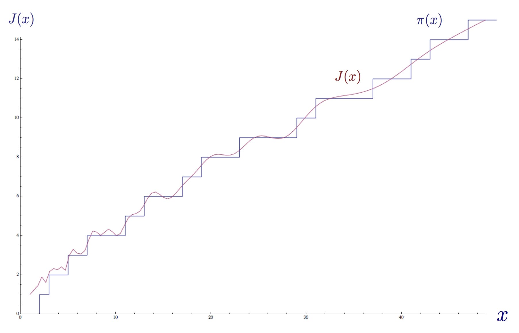
The prime counting step function π(x) being approximated by the explicit formula for the Riemann prime counting function J(x) using the first 35 non-trivial zeros ρ of the Riemann Zeta function.
In the chart above, I have approximated the prime counting function π(x) by using the explicit formula for the Riemann prime counting function J(x), and summed over the first 35 non-trivial zeros of the Riemann zeta function ζ(s). We see that the periodic term causes the function to “resonate” and begin to approach the shape of the prime counting function π(x).
Below you can see the same chart, using more non-trivial zeros.
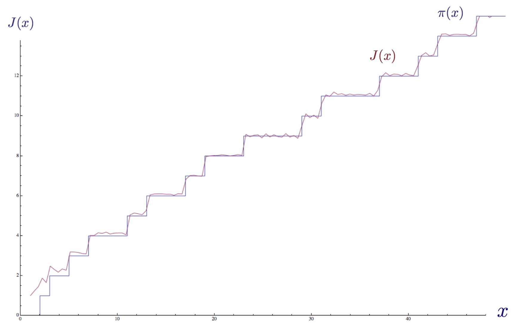
The prime counting step function π(x) being approximated by the explicit formula for the Riemann prime counting function J(x) using the first 100 non-trivial zeros ρ of the Riemann Zeta function.
Using Riemann’s explicit function, one can approximate the number of primes up to and including a given number x to a very high accuracy. In fact, Von Koch proved in 1901 that using the non-trivial zeros of the Riemann zeta function to error-correct the logarithmic integral function is equivalent to the “best possible” bound for the error term in the prime number theorem.
“..These zeros act like telephone poles, and the special nature of Riemann’s zeta function dictates precisely how the wire — its graph — must be strung between them..”
Epilogue
Since the death of Riemann in 1866 at the modest age of 39, his groundbreaking paper has remained a landmark in the field of prime- and analytic number theory. To this day Riemann’s hypothesis about the non-trivial zeros of the Riemann zeta function remains unsolved, despite extensive research by numerous great mathematicians for hundreds of years. Numerous new results and conjectures associated with the hypothesis are published each year, in the hope that one day a proof will be tangible.
Thank you for reading Privatdozent. If you are interested in learning more about the Riemann hypothesis, I recommend starting with Quanta Magazine’s video before moving on to the books I recommend in this previous newsletter:
PrivatdozentThe Best Books on: The Riemann Hypothesis
Hi there. Around 2010, as an undergraduate in mathematics I fell absolutely in love with the Riemann hypothesis (RH), as one does. I spent Friday nights researching, reading and trying to understand this most famous of all math problems. In the process, I accrued a bundle of books on the topic. Some were better than others. The following are the ones I would recommend to another 21-year-old interested in understanding the Riemann zeta function, its properties and the implications of Riemann’s hypothesis for the distribution of prime numbers…Read more
The Privatdozent newsletter currently goes out to 8,123 subscribers via Substack.
References
No comments:
Post a Comment